How Many Pressure Gauges Does It Take to Pin a Leak to One Pipe? A Full Walk-Through of the Pressure-Fingerprint Method
Leaks are buried underground; digging up the whole network to find them is a non-starter. Yet a handful of pressure gauges already carry the location signal in their readings. This article works the full method — from raw pressure readings to a ranked list of candidate leak pipes — from hydraulic first principles, number by number, on a single 6-node teaching network.
Scope note: every number below comes from a 6-node teaching network (one reservoir at 40 m head, 6 nodes, 7 pipes) run as a synthetic experiment. It is meant to teach the mechanism and the sensor-placement rules, not to report any real network's field results. Single-leak assumption throughout; measurement noise synthesized at σ=0.02 m (±2 cm gauge precision). Small as it is, the demo network keeps the structure that matters — looped supply, pipe-diameter variation, and the trunk-vs-branch distinction. Once the method is clear here, scaling up only enlarges the matrices; the chain is unchanged.
▶ Interactive version (run the Monte-Carlo live): both live demos in this article — single-shot localization and the 18,000-inversion sensor-ladder experiment — can be clicked and recomputed on the spot. Nothing is a canned image. Open it alongside the matching sections.
1. The problem: leak hunting is a funnel, and this method sits in the middle
In water-network leak management, "where is it leaking" is the most expensive question. The full hunt is a funnel that narrows stage by stage, each using different physics and hardware:
- Detect — is there a leak, how much: bulk-meter reconciliation, DMA night-minimum-flow analysis. If the books don't balance, there is a leak. Uses flow.
- Localize (this method) — which pipe: pressure-fingerprint matching, collapsing all candidates into a top-K probability list, shrinking the search from the whole network to two or three pipes. Uses pressure.
- Pinpoint — which meter along the pipe: acoustic loggers / noise correlators. Uses acoustics.
- Repair — excavate: the span is already down to meters, so digging cost is controlled.
Pressure and flow have distinct, non-interchangeable roles in this funnel:
| Flow (bulk reconciliation) | Pressure (multi-point pattern) | |
|---|---|---|
| Question answered | Is there a leak, how much (detect) | Which pipe (localize) |
| Information form | A single total, no spatial distribution | The spatial distribution of drawdown — the carrier of location |
| Device economics | Flow meters are expensive, only at boundaries | Pressure gauges are cheap, can be spread inside the network |
| Blind spot | Can't localize (boundary sees only totals) | Trunk-type uniform-drawdown leaks (see the P0 blind spot, ch. 7) |
So the first-layer answer to "why localize with pressure not flow" is the division of labor: flow already confirmed "there is a leak" at stage ①; stage ② needs spatial information, and spatial information lives only in densely placed pressure gauges. The deeper physical answer comes in chapter 5.
Localization is the "expensive" question precisely because it is sandwiched between two cheap stages: detection just reads a bulk meter, repair just opens the confirmed span. Only "which pipe of the whole network" has no directly readable instrument — the buried network is invisible. The value of the fingerprint method is turning that invisible middle into an actionable suspect list using cheap sensors plus a hydraulic model.
The mathematical form: readings in, ranked probabilities out
M is the number of gauges, N the number of candidate leak sites (here M=3, N=7; in the field N is the count of candidate pipe segments). Why a ranked probability, not a coordinate? Three reasons:
- The information doesn't add up: M readings carry limited information — chapter 7 shows only M−1 dimensions survive de-meaning — so pinning a unique continuous coordinate is wishful. The honest output is "which pipes are most suspect, and how confident."
- The downstream use is a checklist: stage ③ walks the top-K list pipe by pipe. A ranked probability is exactly its input format.
- Failure is observable: probability carries confidence. A top-1 leading by 70 points versus by 0.3 points are completely different action cues (the latter is a coin flip, as we'll see). A coordinate-only black box can't tell you that.
The whole chain is four steps: build the fingerprint library (offline, once) → compute residual → de-meaned Pearson match → softmax probability. The rest of the article works every step's numbers to the end.
2. The demo network and the minimal hydraulics
Full parameters
One waterworks (reservoir boundary, fixed head 40.00 m, the only pressure boundary) feeds the network via trunk P0; P1–P6 form a loop. Six nodes J1–J6, each with user demand 0.004 m³/s (≈4 L/s), 0.024 m³/s total; all node elevations are 0 — so head H = gauge reading p throughout.
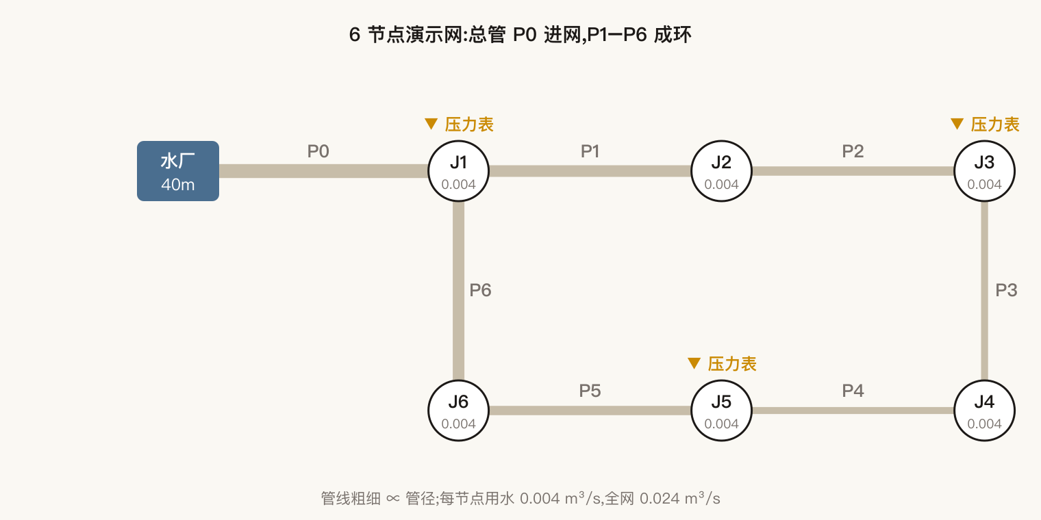
Pipe resistances R (roughness C=100 network-wide):
| Pipe | Between | L (m) | D (m) | R (m/(m³/s)^1.852) |
|---|---|---|---|---|
| P0 | Works–J1 (trunk) | 150 | 0.30 | 111.4 |
| P1 | J1–J2 | 250 | 0.25 | 451.5 |
| P2 | J2–J3 | 400 | 0.20 | 2 141.8 |
| P3 | J3–J4 | 200 | 0.15 | 4 348.4 |
| P4 | J4–J5 | 500 | 0.15 | 10 871 |
| P5 | J5–J6 | 300 | 0.20 | 1 606.4 |
| P6 | J6–J1 | 180 | 0.25 | 325.0 |
The one equation you need
The whole method rests on one empirical hydraulic law. Water rubbing against pipe walls loses energy along the way, seen as head (= pressure here, since elevation is 0) declining. The head lost in one pipe is the friction loss h, given by Hazen-Williams:
In SI (Q in m³/s, D and L in m, h in m), the constant 10.667 holds. The exponent 1.852 is the key nonlinearity: double the flow and loss grows ×, not 2× — turbulent friction. And D's −4.871 power is brutally sensitive: halve the diameter and R rises ≈29×.
Work trunk P0 end to end (L=150 m, D=0.30 m, C=100; reservoir 40 m; all 0.024 m³/s enters through it):
- ① R =
- ② h = m
- ③ m
That's all — the gauge at J1 should read 39.889 m. Feel the nonlinearity: double demand to 0.048 m³/s and loss becomes m, 3.61× not 2×. Add one more piece of common sense — node conservation: a node stores no water, so at any instant "inflow = outflow + local demand." One equation plus one rule is the entire hydraulics.
3. The baseline: 13 unknowns, solved by hand and checked against the simulator
With no leak, the unknowns = 6 node heads + 7 pipe flows = 13. Three steps.
Step 1, the total. All 0.024 m³/s comes from the works, so m³/s — just bookkeeping. 12 left.
Step 2, node-by-node accounting. Let P1's flow be (J1→J2), then walk the loop with "in = out + local":
| Node | Balance | Yields |
|---|---|---|
| J1 | in 0.024, use 0.004, send via P1, rest via P6 | |
| J2 | in , use 0.004 | |
| J3 | in , use 0.004 | |
| J4 | in , use 0.004 | (negative = reverse flow) |
| J6 | in , use 0.004 | |
| J5 | check: | exactly = 0.004 ✓ |
The last row's cancels — 6 conservation balances have only 5 independent; one more equation must come from energy. Now just 1 unknown, .
Step 3, close with energy. From J1 to J4 there are two paths; J1 and J4 each have one head, so total loss along the two paths must be equal:
With and no closed-form root for the 1.852 power, iterate:
| try (m³/s) | upper (m) | lower (m) | verdict |
|---|---|---|---|
| 0.008 | 0.137 | 0.694 | upper loss too small → more water to upper → larger |
| 0.012 | 0.563 | 0.101 | overshoot → smaller |
| 0.010 | 0.297 | 0.297 | equal ✓ (exact root 0.0099975; 0.010 is enough by hand) |
Now roll head down from 40 m pipe by pipe:
| Solve | Path | h substitution | by hand H (m) | sim (m) |
|---|---|---|---|---|
| J1 | 40 − h([email protected]) | 111.4×0.001000 = 0.111 | 39.889 | 39.8885 |
| J2 | J1 − h([email protected]) | 451.5×0.000198 = 0.089 | 39.800 | 39.7993 |
| J3 | J2 − h([email protected]) | 2141.8×0.0000768 = 0.164 | 39.636 | 39.6350 |
| J6 | J1 − h([email protected]) | 325.0×0.000198 = 0.064 | 39.825 | 39.8242 |
| J5 | J6 − h([email protected]) | 1606.4×0.0000768 = 0.123 | 39.702 | 39.7008 |
| J4 | J5 − h([email protected]) | 10871×0.0000100 = 0.109 | 39.593 | 39.5915 |
Max hand-vs-sim gap is 0.002 m, all from display rounding; at full precision the chain matches the simulator to four decimals — hand and simulator solve the same equations, no black box. The baseline the three gauges (J1/J3/J5) see (using the simulator's exact values hereafter):
The entire game of leak detection is subtracting new readings from this row.
4. Modeling the leak: 16 coupled equations
Split the pipe, drill a hole — the leak flow is solved for
A pipe is a line; you can't drill a hole on it, so a small surgery (split_pipe): cut the pipe at its midpoint, spawn a virtual node LEAK there, drill on it. For P5 (J5–J6, 300 m):
R is proportional to length, so 1606.4 splits into 803.2 per 150 m half. The hole has two parameters: area A = 0.001 m² (≈3.6 cm) and discharge coefficient Cd = 0.75.
How much sprays out? Torricelli: jet speed equals free-fall speed from "that pressure-head high," , so
Crucially is unknown (the pressure there once the hole is open must be solved), so is unknown too. You give the model only the hole's geometry (A, Cd); how much leaks is what it computes. Because leak and demand both vary with pressure, the simulation must run in pressure-driven (PDA) mode: drawdown suppresses leak and demand, which feeds back into pressure — a loop only PDA captures. Demand follows Wagner's three-segment law (full above 21 m, zero below 3.5 m, in between); here pressure stays above 38 m so reduction never activates, but the equation is always in the system.
Solving the 16 equations
With P5 open, the unknowns become 16: 7 node heads (incl. ) + 8 pipe flows (P5 split) + 1 leak flow. Exactly 16 equations: 7 node conservation + 8 pipe energy + 1 orifice — closed. Nonlinearity from the 1.852 power and the square root means no closed form — the simulator uses Newton iteration. Key numbers of the converged solution:
| Quantity | Value | Read |
|---|---|---|
| Leak | 0.02063 m³/s | ≈86% of normal 0.024 demand — a deliberately large hole, clear signal |
| Leak head | 38.5529 m | check: m/s (≈99 km/h), ✓ |
| Trunk flow | 0.04463 m³/s | = 0.024 + 0.02063; trunk loss rises 0.111 → 0.352 m |
| P5 segment direction | 0.00178 (J5→LEAK) | the far path reverses to feed the hole — direction is solved, not set |
All 16 equations close on back-substitution (±0.0003 m residues are table rounding). Subtracting post-leak pressures from the baseline node by node gives this chapter's product — the drawdown vector Δp:
| J1 | J2 | J3 | J4 | J5 | J6 | |
|---|---|---|---|---|---|---|
| baseline (m) | 39.889 | 39.799 | 39.635 | 39.592 | 39.701 | 39.824 |
| post-leak (m) | 39.648 | 39.477 | 39.036 | 38.679 | 38.546 | 39.260 |
| Δp (m) | 0.240 | 0.322 | 0.599 | 0.913 | 1.154 | 0.564 |
The rule is visible: the closer to the hole, the bigger the drop (hole between J5–J6, J5 drops 1.154 m; J1 near the works only 0.240 m). This spatial pattern of drawdown is the "fingerprint."
5. The fingerprint library: precompute what each pipe's leak looks like
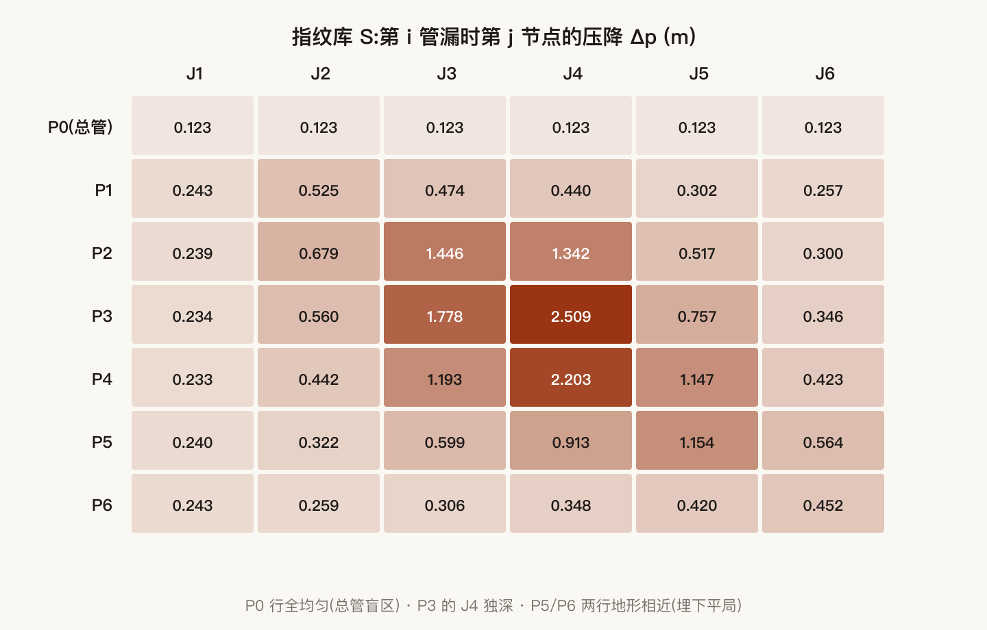
Repeat the P5 routine — inject, solve, subtract from baseline — for every candidate pipe, stack 7 rows into a matrix:
Here N=7, all 6 nodes computed (installing k gauges = masking columns at match time). The 7×6 library:
| Leak pipe | J1 | J2 | J3 | J4 | J5 | J6 |
|---|---|---|---|---|---|---|
| P0 | 0.123 | 0.123 | 0.123 | 0.123 | 0.123 | 0.123 |
| P1 | 0.243 | 0.525 | 0.474 | 0.440 | 0.302 | 0.257 |
| P2 | 0.239 | 0.679 | 1.446 | 1.342 | 0.517 | 0.300 |
| P3 | 0.234 | 0.560 | 1.778 | 2.509 | 0.757 | 0.346 |
| P4 | 0.233 | 0.442 | 1.193 | 2.203 | 1.147 | 0.423 |
| P5 | 0.240 | 0.322 | 0.599 | 0.913 | 1.154 | 0.564 |
| P6 | 0.243 | 0.259 | 0.306 | 0.348 | 0.420 | 0.452 |
Three reading rules everything downstream grows from:
- Each row is a "terrain": P3 leaking drops J4 by 2.509 m (adjacent) but J1 only 0.234 m. Distance decay holds in every row; differing terrains are the source of distinguishability.
- Some rows look alike: P5 and P6 both read "J5/J6 side drops more, J1 side less," differing only in magnitude — the tie of chapter 6 is already seeded here.
- P0's row is flat: a trunk leak drops all six nodes uniformly by 0.123 m. Uniform = no spatial pattern = nothing for any matcher to grab (the structural blind spot, chapter 7).
Three engineering properties: offline once (N sims, built before any leak; online localization runs no hydraulics, just vector matching, milliseconds); fixed hole is fine (matching looks only at shape not magnitude, so one library handles all leak sizes); library quality is capped by model quality (bad roughness/diameter → distorted fingerprints; field roughness must be calibrated against measured pressure).
The physics: drawdown pattern is the "shadow" of flow redistribution
The full causal chain when a leak appears: hole opens → pipe flows redistribute (works supplies more, flows re-split by resistance, some pipes even reverse) → each pipe's flow changed, so its loss changed → node heads shift. So the spatial drawdown pattern = the shadow of flow redistribution projected through the energy equations. Matching on pressure isn't discarding flow information — the spatial flow change is already encoded into the pressure field. We read, with cheap gauges, what only expensive flow meters could directly measure.
6. Matching: residual → de-mean → Pearson → softmax
Switch to the online moment: P5 is leaking (we pretend not to know); three gauges report.
Step 1: the residual r
| Gauge | baseline (m) | measured (m) | residual r (m) |
|---|---|---|---|
| J1 | 39.889 | 39.648 | 0.240 |
| J3 | 39.635 | 39.036 | 0.599 |
| J5 | 39.701 | 38.546 | 1.154 |
The teaching version uses zero-noise "perfect readings" (the converged solution at the three gauge sites). Note r is exactly the J1/J3/J5 columns of P5's fingerprint row — a basic self-consistency check. The question is one sentence: which of the 7 rows looks most like r?
▶ From here, the "single-shot" demo in the interactive version is best read hands-on: click any pipe to set the leak, and the probability bars recompute by exactly this algorithm.
Step 2: don't compare directly — de-mean first
The naive move is cosine similarity of r against each row. It fails: a leak makes all three gauges drop (r all positive), and every library row is all positive too — every vector points "all down," cosines all >0.95, everyone "looks alike." Signal processing calls this common-mode swamping the differential mode.
The fix is de-meaning — subtract the shared "everyone drops," keep only "who drops more/less than average":
Which reads: "J1 drops 0.42 below average, J5 drops 0.49 above" — the location signature, independent of leak size.
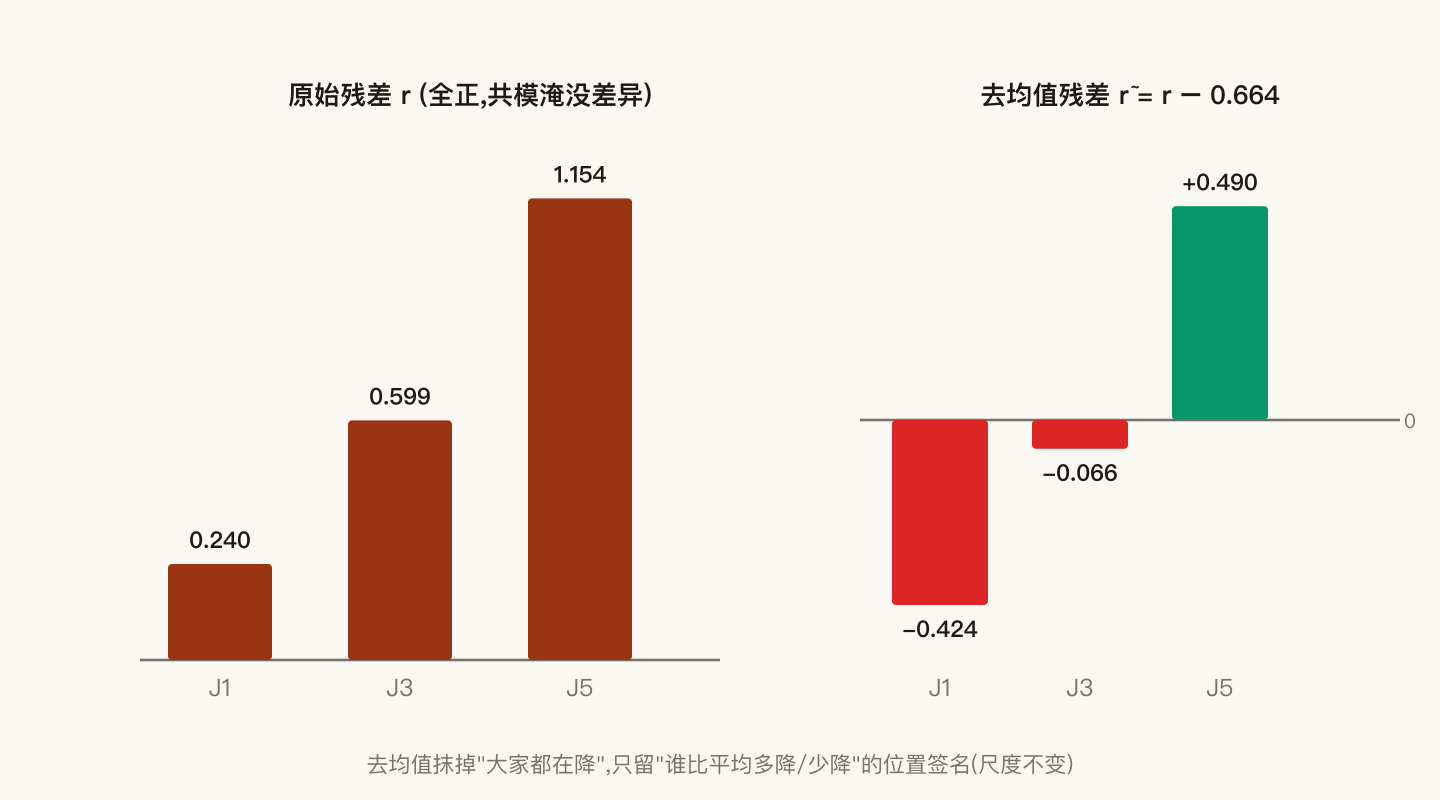
The second dividend of de-meaning is scale invariance: a bigger hole scales r nearly proportionally, so after de-mean + normalize the direction is unchanged — matching needs no prior on leak size. The cost is buried here too: de-meaning eats one degree of freedom, leaving M gauges only M−1 dimensions.
Step 3: de-meaned cosine = Pearson correlation
Numerator m², denominator m×m, units cancel, score is dimensionless — matching sees only pattern direction, not magnitude. Work P6's row by hand (chosen because its result is the most surprising):
- ① P6 fingerprint (J1/J3/J5) = [0.243, 0.306, 0.420], mean 0.323, de-meaned
- ② dot =
- ③ norms ;
- ④ score =
That 0.999: P6 isn't leaking, yet its correlation with the residual is near perfect. Its de-meaned direction ("J1 less, J5 more") is nearly identical to the true culprit P5, differing only in magnitude — which scale invariance erased. Not an error: from three gauges the two pipes physically look the same. Pearson honestly reports high similarity for genuinely similar shapes; it won't invent a distinction that isn't there.
Step 4: softmax turns 7 scores into 7 probabilities
β is a display dial amplifying "score gaps" into "probability gaps" — a monotone transform that doesn't change ranking, only display contrast. All seven pipes (de-meaned fingerprint, Pearson, , softmax; intermediates to 3 decimals):
| Pipe | de-meaned (m) | Pearson | softmax | |
|---|---|---|---|---|
| P0 | [0, 0, 0] ← flat → zero | ~0 | 1.1 | 0.0% |
| P1 | [−0.097, +0.134, −0.037] | +0.126 | 2.7 | 0.0% |
| P2 | [−0.495, +0.712, −0.217] | +0.098 | 2.2 | 0.0% |
| P3 | [−0.689, +0.855, −0.166] | +0.215 | 5.6 | 0.1% |
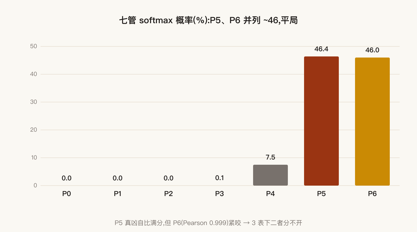
| P4 | [−0.624, +0.335, +0.289] | +0.772 | 479.7 | 7.5% |
| P5 | [−0.424, −0.066, +0.490] | +1.000 | 2981.0 | 46.4% |
| P6 | [−0.080, −0.017, +0.097] | +0.999 | 2958.7 | 46.0% |
| Σ = 6431 | 100% |
The denominator: , so , , .
Reading the tie: a nominal hit = a coin flip
With 3 gauges, P5 truly leaking, full-machine computation (no intermediate rounding) gives 46.3% : 46.0% [footnote ★]. Two readings, vastly different:
- Wrong: "top-1 is P5, hit." — great-looking top-1 hit rate that hides the real decision state.
- Right: "P5 and P6 are inseparable; picking one is a coin flip; both must be inspected." — a 0.3-point lead vanishes under any noise.
★ Footnote (cross-check): the hand-computed figure (intermediates to 3 decimals) is 46.4% : 46.0%, the full-machine figure is 46.3% : 46.0% — the 0.1 pp difference is purely rounding-digit choice, corroborating rather than contradicting. Both are kept to make the point: this difference doesn't affect the ranking; P5/P6 are simply inseparable.
Side by side, the de-meaned fingerprints P5 [−0.424, −0.066, +0.490] and P6 [−0.080, −0.017, +0.097] are the same direction, different magnitude; their mutual Pearson = 0.9991. Physically both hang on the loop's lower-left; from three gauges their relative patterns are almost identical, and the magnitude difference is erased by scale invariance. From three gauges they are physically inseparable; 46:46 is the honest output — the live proof that the output must carry confidence. Why exactly three, and which gauge fixes it? That's the degrees-of-freedom account next.
7. Degrees of freedom and the sensor ladder: how many, and where
The DoF account: M gauges give only M−1 resolving dimensions
De-meaning isn't free: after subtracting the shared mean, components sum to zero — the vector is pressed into an (M−1)-dimensional subspace:
| Gauges M | Dims M−1 | Geometry |
|---|---|---|
| 3 | 2 | 7 fingerprint directions crammed into one 2-D plane — collisions are inevitable |
| 2 | 1 | one axis; each fingerprint degenerates to a single ratio ("J1 vs J5, who drops more") |
| 1 | 0 | a number minus its own mean is 0; residual is the zero vector — mathematically always blind, not "fuzzier" |
Here 3 gauges = a 2-D plane holding 7 directions, so more than one collision. P5/P6 is one; adding a gauge = adding a dimension. Their difference hides in column J6 (0.564 vs 0.452 m), and J6 had no gauge — install it and the fingerprints go 3-D → 4-D, the new component being −0.075 vs +0.096 (opposite signs, split apart), Pearson falls 0.9991 → 0.657, output flips 46:46 → P5 alone at 83.4%. Insufficient dimensions can't separate collinear candidates no matter how clever the algorithm — an information-theoretic limit, not an algorithm flaw.
A per-scenario table, each pipe set as the true leak, zero-noise top-1 confidence and lead (3 gauges vs all-6):
| True leak | 3-gauge baseline (J1/J3/J5) | all 6 gauges |
|---|---|---|
| P0 | 14.3% (0.0 pp, blind) | 14.3% (0.0 pp, blind) |
| P1 | 32.5% (0.1 pp) | 85.9% (74.9 pp) |
| P2 | 32.9% (0.1 pp) | 53.1% (22.6 pp) |
| P3 | 32.3% (1.1 pp) | 44.8% (17.3 pp) |
| P4 | 59.4% (48.6 pp) | 52.5% (20.2 pp) |
| P5 | 46.3% (0.3 pp) | 83.3% (74.6 pp) |
| P6 | 47.0% (0.3 pp) | 92.6% (85.4 pp) |
Key finding: it isn't only P5/P6 tied — the upper path P1/P2/P3 are triplets too (leads of just 0.1 pp). A 2-D plane with 7 directions produces collisions in two groups at once. Also note all-6's P4 confidence is lower than 3-gauge (52.5 < 59.4) — confidence is a relative quantity; adding gauges reshapes all candidates' geometry, so an individual scenario's displayed confidence can fall while hit ability does not.
The sensor ladder: performance as gauges go 6→1
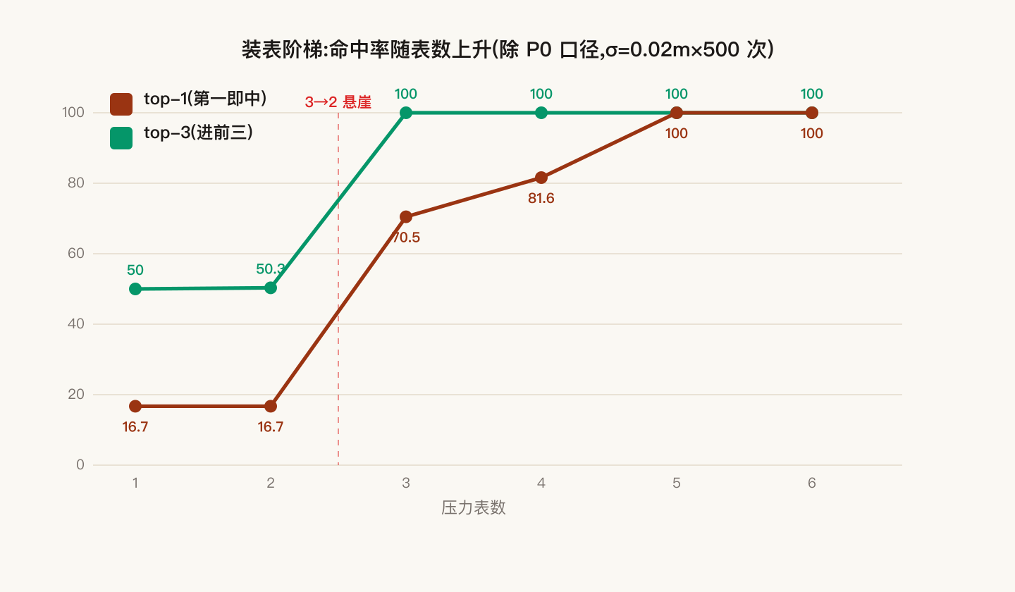
The engineering question: how many gauges are enough? A clean controlled experiment: the 7×6 library stays fixed ("k gauges" = mask columns; single variable, clean attribution); the algorithm is unchanged; each reading gets N(0, σ=0.02 m) noise (±2 cm is typical online-gauge precision; without noise the hit rate inflates); 500 independent draws per scenario (±2 pp binomial jitter); a nested add-order (J5 ⊂ J1/J5 ⊂ J1/J3/J5 ⊂ +J6 ⊂ +J2 ⊂ +J4); top-1 / top-3 hit rate, excluding P0 (always blind, a constant drag on every tier).
▶ This whole ladder can be run "live" in the interactive version — the browser does 6 tiers × 6 true-leak scenarios × 500 noisy draws (18,000 inversions), reproducing the reference within ±3 pp on a fresh seed. That is the on-the-spot proof the numbers aren't invented.
Main ladder:
| Gauges | Points | True P5: top-1 & conf | Lead | Noisy top-1 (ex-P0) | Noisy top-3 (ex-P0) |
|---|---|---|---|---|---|
| 6 | J1–J6 all | P5 83.3% | 74.6 pp | 100.0% | 100% |
| 5 | −J4 | P5 78.7% | 66.0 pp | 100.0% | 100% |
| 4 | base +J6 | P5 83.4% | 72.6 pp | 81.6% | 100% |
| 3 | base J1/J3/J5 | P5 46.3% | 0.3 pp (coin flip) | 70.5% | 100% |
| 2 | J1/J5 | P5 16.7% | 0.0 pp | 16.7% | 50.3% |
| 1 | J5 | P6 14.3% (=1/7 guess) | 0.0 pp | 16.7% | 50.0% |
Three kinks on the ladder
- 3 → 2 is a cliff, not a slope. 3 gauges still have 2 usable dims (ex-P0 top-1 70.5%, top-3 100%); 2 gauges leave 1 dim — each fingerprint degenerates to one ratio, top-1 collapses to 16.7% (≈1/6 guess), top-3 down to 50%.
- 1 gauge = mathematically always blind, not "fuzzier." A number minus its own mean is 0; the residual is the zero vector; probability stays 1/7 forever. A single gauge does only "pressure is low" alarming, zero localization. The absolute floor: at least two to participate, at least three for usable accuracy.
- The 6th gauge (J4) is wasted. 5 and 6 gauges have identical noisy hit rates (ex-P0 both 100%) — J4's information is sandwiched by J3/J5, essentially redundant. More is not better; enough to separate all confusion pairs is the ceiling.
Read together, the decision rule: from the floor up, each added gauge asks "which confusion pair did it split" — split, add; can't, stop. This network's answer is 4 (top-1 81.6%, top-3 100%). The values change with the network, but the "diminishing returns + a clear ceiling" curve shape is universal.
This curve is itself the correct deliverable of a sensor-count argument. Reviews often argue "3 or 5" with no basis; run this ladder and the discussion shifts from guessing numbers to reading a curve.
Which 4th gauge: position > count
Fixing the 3-gauge baseline, three ways to add a 4th (all machine-computed):
| Option | True P5: conf / lead | Noisy top-1 (ex-P0) | Splits | Doesn't split |
|---|---|---|---|---|
| +J6 | 83.4% / 72.6 pp | 81.6% | P5/P6 (0.3 → 72.6 pp) | upper P1/P2/P3 still crammed |
| +J2 | 45.0% / 0.3 pp | 88.5% | upper triplets | P5/P6 still a coin flip |
| +J4 | 50.3% / 4.6 pp | 87.5% | upper triplets (partly) | P5/P6 mostly still mixed |
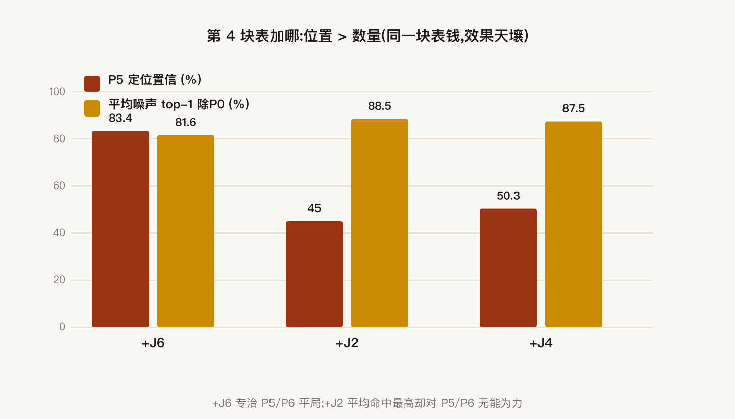
Three distinct personalities: +J6 cures P5/P6 but not the upper triplets; +J2 tops average hit (88.5%) but leaves P5/P6 a coin flip; +J4 sits in between. No free universal 4th gauge. So the placement order is nailed down: simulate to find confusion pairs first → place by "which to split," not by even geometric spread. A counter-intuitive detail: 5-gauge P5 confidence (78.7%) is lower than 4-gauge (83.4%) — adding an uninformative gauge dilutes display contrast but doesn't lower hits (5-gauge top-1 still 100%). Confidence is relative; judge by hit rate.
The P0 blind spot: an information-theoretic certainty
P0's row is flat: all six nodes drop uniformly 0.123 m. Uniform drawdown de-means to the zero vector — no spatial pattern for any matcher. Not a flaw but a certainty: the trunk sits between source and network, so its leak is "the whole source head shifting down," felt identically everywhere; any number of gauges stays blind. The backstop returns to funnel stage ①: a trunk leak hides in the pressure pattern but not the flow total — works output surges without matching district metering, and DMA night-minimum flow exposes it. So a complete scheme has two legs: branch/loop leaks (with spatial pattern) localized by pressure fingerprints; trunk-type uniform leaks caught by flow reconciliation. The two blind spots are complementary — pressure localizes, flow detects.
8. Boundaries, conclusions, and Q&A
Honest boundaries
- Teaching network: all numbers from a 6-node zero-/added-noise synthetic; it shows mechanism and curve shape, not field results.
- Single-leak assumption: multiple simultaneous leaks superpose fingerprints; single-fingerprint matching may point at an innocent middle pipe.
- Zero-model-error assumption: fingerprints are model-computed; wrong roughness/diameter distorts them. Trustworthiness requires a network model calibrated against measured pressure.
- Demand fluctuation not modeled: real demand varies; the field fix is to measure during night-minimum-flow hours and average multiple readings.
When the method fails is set by signal-to-noise. Here the leak is large (0.02063 m³/s ≈86% of demand), the max signal 1.15 m ≫ σ=0.02 m, so even 3 gauges hit 70%. Smaller/farther leaks weaken the signal; when fingerprint amplitude falls to noise level, scores flatten and top-1 reverts to guessing. This doesn't change the method's role — a mid-funnel range-narrowing tool (top-K list + field confirmation), not a one-shot instrument.
Conclusions
- Role: outputs a top-K list, shrinking whole-network search to two or three pipes; the confidence (lead) is itself an action cue.
- Count: not more-is-better. Here 4 gauges split the target pair (top-1 81.6%, top-3 100%), the 6th is wasted, 3→2 is a cliff, below 2 the method fails. Argue with the whole marginal-benefit curve, not a single number.
- Position > count: the same gauge, right (+J6) vs wrong position is 72.6 pp vs 4.6 pp on the target pair. Correct flow = simulate confusion pairs first, then place.
- Blind spot & backstop: trunk-type uniform leaks are structurally immune to pressure-pattern methods and must be complemented by flow reconciliation — pressure localizes, flow detects, both legs required.
Q&A (anticipated challenges)
Q1 · How is β=8 set? Does changing β change conclusions? β amplifies score gaps into probability gaps; a monotone transform doesn't change the ranking, so top-1 and hit rate are β-independent. 8 is a display value; for calibrated probabilities, fit β to historical validation data.
Q2 · The library uses a fixed 0.001 m² hole; what about other leak sizes? De-meaned Pearson looks only at shape, not magnitude (scale invariance); a bigger hole scales all drawdowns proportionally, shape unchanged, one library covers all. This approximation degrades for very large leaks that heavily activate the PDA reduction zone — a known boundary.
Q3 · Why must the simulation be PDA? Is the leak flow an input? Leaking is a coupled problem: drawdown suppresses leak and demand, feeding back into pressure until equilibrium — a loop only PDA expresses. The leak flow is not an input; you give only the hole geometry (A, Cd), and how much leaks is solved from leak-point pressure via the orifice equation (0.02063 m³/s closes on back-substitution).
Q4 · Does the model need "initial conditions"? Two layers. System level: no — no tanks, no storage states, it's an algebraic system, not a differential one; no "t=0 state." Solver level: yes but built-in — Newton's starting point is internal (head=elevation, pipe flow=0.001 m³/s, etc.), affecting only convergence speed, not the solution, which the equations fix uniquely.
Q5 · What does top-3 = 100% mean, and why is it more relevant than top-1? Stage ③ walks suspect pipes one by one. top-3 = 100% means inspecting the top three necessarily catches the culprit — workload capped at 3 of 7 pipes. The 3-gauge top-1 is only 70.5% but top-3 is already 100%, so "are 3 gauges enough" depends on the workload you accept.
Q6 · Moving to a bigger network — what changes, what doesn't? Unchanged: the four-step chain, the DoF account (M gauges, M−1 dims), the "find confusion pairs then place" logic, the P0-type blind spot / flow-reconciliation complementarity. Changed: the candidate set becomes N pipe segments (bigger matrices); the library must be rebuilt on a calibrated model; confusion-pair structure follows the real topology and must be re-simulated; noise is set by actual gauge precision and demand fluctuation. The methodology transfers whole; every number is recomputed.
In one line: how many gauges it takes to pin a leak to one pipe is no mystery — it's set by one Hazen-Williams equation, one de-meaned Pearson match, and an (M−1)-dimensional degrees-of-freedom account. How many, and where, shouldn't be guessed but read off the marginal-benefit curve above. Both live demos can be rerun on the interactive page, and every intermediate number is out in the open for you to check.