WRITING
Unpack the Coupon and There Are Only Two Kinds of Money: Treasury Interest, and Insurance Premium

The previous post reconciled a 7x gap: a buy-write note with a 21.6% annualized face rate whose model expectancy is barely 3%. That post answered "why is expectancy below naked stock, and is it still worth running?" This one digs deeper, into two harder questions:
One: why is the EV pinned near T-bills, exactly? Is it poor strike selection — would another strike or another underlying do better? Two: how big is the tail? What's the probability of breaching break-even, how much do you lose when you do, and where does the model stop being trustworthy?
Every number comes from the real option chain frozen at the 2026-07-17 close (QQQ 743.29) and 27 years of daily history; scripts reproducible, zero mental math.
0. Conclusions first
| Question | Answer |
|---|---|
| EV ≈ T-bills — did I pick badly? | No. It's a structural consequence of no-arbitrage pricing: coupon = treasury interest + put insurance premium, and the premium's expected payout ≈ the premium itself. True at every strike, on every underlying |
| Would SPY be better? | Not "better value" — just a different shape: SPY's low IV means the same 15% coupon floor buys only a 3.3% cushion (QQQ gives 8.6%); but SPY's tail is genuinely thinner |
| How big is the tail? | Per note: P(net loss) ≈ 24%; conditional on losing, the average loss is ~5% of capital (≈ 2.5 coupons); the worst 35-day window in history maps to ~−26% of capital |
| Is the model trustworthy? | Conservative in the mid-range, optimistic ~5x in the extreme tail (at the −25% level: empirical 0.54% vs model ~0.1%) — the fat tail is real; never use model odds as crash protection |
| Where's the real risk? | Often not in the note but in the account: the note's tail settles at expiry; a margin call doesn't wait. The structure is controllable, leverage stacked on top is not |
1. Anatomy of a note: what exactly did you sell?
One real fill: buy QQQ @693.08, simultaneously sell the 35-day 660 call for 46.50. P&L at expiry (per share):
Three symbols: = QQQ's price at expiry; = the strike (the cap); = break-even. At you collect the full 13.42 coupon; below 646.58 you lose 1:1, exactly like naked stock, with no protection whatsoever.
The 46.50 premium contains two kinds of money — separating them is the key to the whole post:
| Component | $/share | What it is |
|---|---|---|
| Intrinsic value = 693.08 − 660 | 33.08 | Your own money coming back — you effectively pre-sold a slice of the stock at 660. Not income |
| Time value (the coupon) | 13.42 | What the market actually pays you |
Only the time value is real income. But why must it equal treasury interest + insurance premium? No formula needed — compare two portfolios (all prices from the same instant at the 07-17 close; reconciliation demands one timestamp):
Portfolio A (the note): buy 1 QQQ share for 695.33, sell the 660C for 47.90 → net outlay today 647.43. Two possible endings: QQQ ≥ 660 — the share is called away at 660, you hold 660 in cash; QQQ = S < 660 — the call expires worthless, you hold stock worth S.
Portfolio B (T-bill + short put): deposit 657.73 in short-term treasuries (3.6%; in 35 days it grows to exactly 660), and sell one 660 put for 10.64 (live chain price) → net outlay today 647.09. Same two endings: QQQ ≥ 660 — the put expires, the deposit matures, you hold 660 in cash; QQQ = S < 660 — the put is exercised, you buy stock at 660 paying with the matured deposit, you hold stock worth S.
| Outlay today | Expiry: QQQ ≥ 660 | Expiry: QQQ = S < 660 | |
|---|---|---|---|
| A stock + short 660C | 647.43 | 660 cash | stock worth S |
| B T-bill + short 660P | 647.09 | 660 cash | stock worth S |
Whatever happens at expiry, A and B end identically → their prices today must be nearly identical. The measured gap is 0.34 — portfolio A holds the actual share and collects one QQQ dividend before expiry, worth roughly exactly that. Even the error reconciles. If the gap ever widened, market makers would buy the cheap side and sell the rich side for riskless profit, snapping prices back within seconds. This is textbook put-call parity; forget the formula, remember the table.
Since note ≡ T-bill + short put, the coupon decomposes automatically:
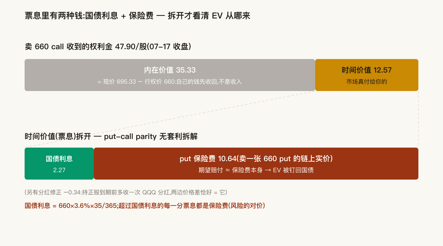
So an ITM-call buy-write is mathematically identical to: deposit K in treasuries + sell one put struck at K for premium. Every cent of coupon above treasury interest is insurance premium. What is the premium's expected payout? That's the next section.
2. Why EV is pinned to treasuries (market structure, not bad picking)
2.1 The closed-loop EV formula
Expected P&L at expiry (per share):
Intuition: pocket the full coupon first; at expiry, for every dollar sits below , you "give back" a dollar — first from the coupon, then from principal. The notation means , so is precisely the fair value of that put — the insurer's expected payout.
Verified on real fills (zero-drift lognormal, = broker closing IV):
| Note (at fill) | Coupon ($/sh) | EV ($/sh) | EV annualized | |
|---|---|---|---|---|
| 680C | 14.00 | 11.67 | +2.33 | +3.5% |
| 660C | 13.42 | 11.63 | +1.79 | +2.9% |
A 21% annualized coupon is fat, but the insurance payout eats it back to ~3% — what's left is almost exactly the treasury-interest term from §1's decomposition. Not a coincidence; the same fact written two ways.
2.2 Why premium ≈ expected payout (who's on the other side)
The QQQ option chain is one of the deepest derivatives markets on earth. Across the table sit market makers who delta-hedge every put they trade in real time — they earn the spread, they don't bet direction. If any strike offered "premium ≫ expected payout," arbitrageurs would sell the structure, hedge it, and lock the difference, forcing the price back to fair. Competition pins every strike's EV to:
VRP (the volatility risk premium) is persistently positive on indices but small (low single digits annualized), and it gets handed back in crash years — it is the normal profit margin of underwriting, not free money.
2.3 Switching strikes doesn't help: every strike slides on the same fair line
On one chain, deep strikes offer high odds and thin coupons, shallow strikes the reverse — the EV column is the same number everywhere. The only thing you truly choose is the shape of the distribution:
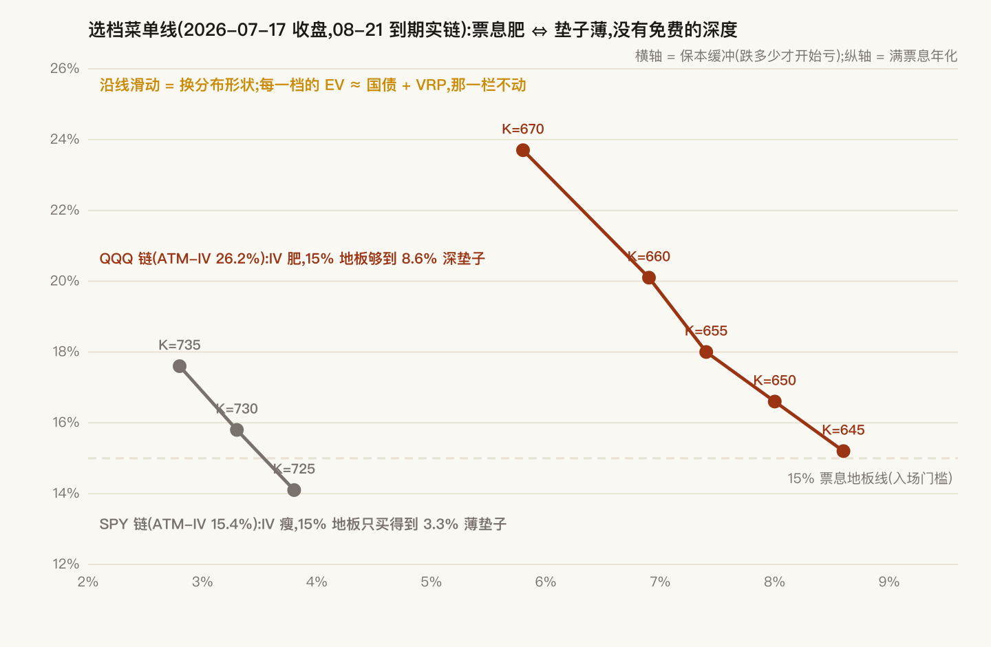
QQQ isn't a bad pick either: tightest spreads, lowest friction. Move to an illiquid single name and friction eats the EV lower still — plus you inherit single-name gap risk.
Then where does CAGR come from? From holding beta itself (the equity risk premium — QQQ's long-run drift of ~+7–10%/yr). The note reshapes that drift into "~76% odds of getting paid monthly," but the drift is the stock's money, not the short call's — selling the call actually gives away the drift above K. That's why the honest benchmark for this defensive structure is treasuries, not QQQ. Whether the trade-off is worth it over full cycles was settled in the previous post: a 25-year replay returns +14.5% cash / +21.7% financed, the excess coming from VRP's historical realization.
3. The tail, computed: how likely, how bad, and how it's done
3.1 Three regions
| at expiry | What happens | Probability (at fill) |
|---|---|---|
| ≥ 660 (K) | Full coupon, +2.08% | 68.7% |
| 646.58–660 (B–K) | Earn less, lose nothing | 7.5% |
| < 646.58 (B) | Net loss, 1:1, unbounded | 23.8% |
3.2 Where the probabilities come from
Model: zero-drift lognormal (deliberately no upward drift — conservative):
Symbol by symbol: = 693.08, the fill price; = 29.6%, the contract's implied volatility; years; a standard normal draw. The key quantity is — one standard deviation of QQQ over 35 days is ±9.2%. Every probability below is measured with this ruler.
The probability of finishing below any level has a closed form ( = standard normal CDF):
Plug in the break-even : , divided by the 9.2% ruler ≈ the break-even sits 0.71 standard deviations out → . That's the whole computation.
3.3 How much do you lose when you lose?
Weight every path below by its probability and the expected net loss also has a closed form — it is the fair value of "a put struck at B":
On the real terms: expected net loss 7.94/share (unconditional); divide by the 23.8% loss probability and the loss-given-loss = 33.31/share ≈ 5.2% of capital. Reading: three times out of four you collect the full coupon; the time you lose, you lose on average ~5% of capital (≈ 2.5 coupons). That's an average, not a bound — the far tail is §4.
3.4 Scenario table (per share, anchored at the 693.08 fill)
| Drop at expiry | Note P&L/sh | Naked stock/sh | Model P(≤ this) | |
|---|---|---|---|---|
| 0% | 693.1 | +13.42 | 0 | 51.8% |
| −5% | 658.4 | +11.85 | −34.65 | 30.4% |
| −6.7% | 646.6 | ≈0 (break-even) | −46.44 | 23.9% |
| −10% | 623.8 | −22.81 | −69.31 | 13.5% |
| −15% | 589.1 | −57.46 | −103.96 | 4.2% |
| −20% | 554.5 | −92.12 | −138.62 | 0.8% |
| −30% | 485.2 | −161.42 | −207.92 | ~0.0% |
Two rules read straight off the table: ① below K the note line and the naked-stock line fall in parallel (slope 1:1), separated by a constant equal to the full 46.50 premium — the cushion's thickness is fixed; it does not thicken as the fall deepens; ② the premium absorbs the first ~6% of decline, but at −30% it recovers only ~22% of the loss. A covered call is not crash insurance — this is the proof.
4. Model vs history: how fat is the tail (27 years of evidence)
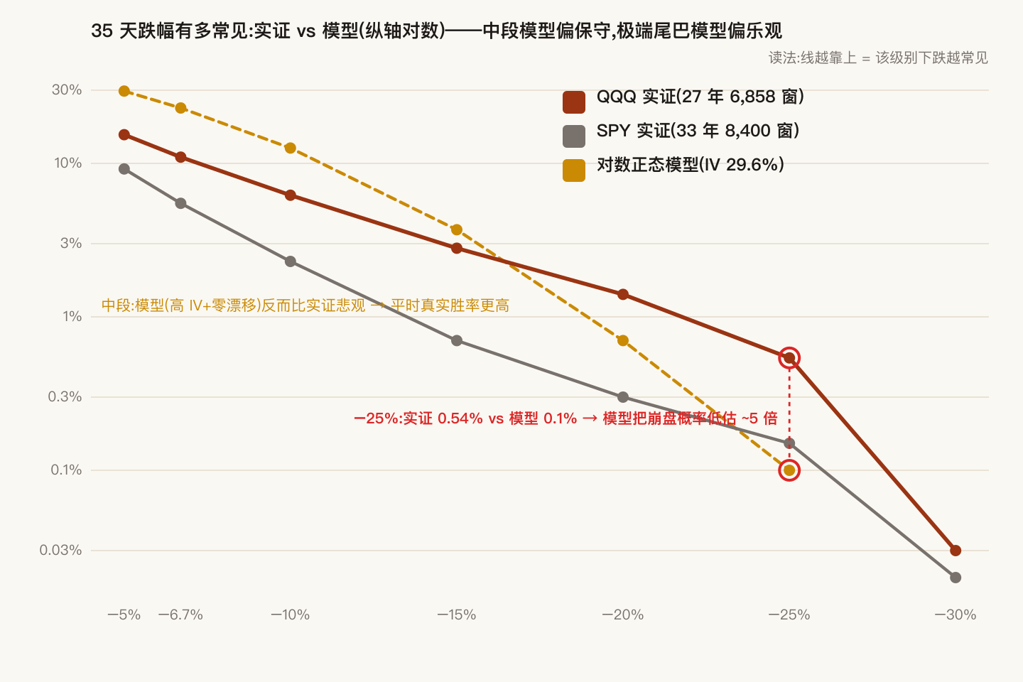
Take every 35-calendar-day window in real history and compare against the model (QQQ 6,858 windows / SPY 8,400):
| 35-day drop beyond | QQQ empirical | SPY empirical | Lognormal model |
|---|---|---|---|
| −5% | 15.4% | 9.2% | 29.6% |
| −6.7% | 11.0% | 5.5% | 23.0% |
| −10% | 6.2% | 2.3% | 12.6% |
| −15% | 2.8% | 0.7% | 3.7% |
| −20% | 1.4% | 0.3% | 0.7% |
| −25% | 0.54% | 0.15% | ~0.1% |
| −30% | 0.03% | 0.02% | ~0.0% |
Two honest conclusions:
- Mid-range, the model is conservative (at −6.7%: model 23% vs empirical 11%): your real-world win rate runs above what the model reports — a built-in margin of safety.
- In the extreme tail the model is ~5x optimistic: the lognormal congenitally understates crashes. Never use model probabilities to make decisions about extreme drops — manage extremes with the scenario table (§3.4) and the worst historical window. Worst 35-day windows on record: QQQ −31.2% (once in 2001-02, once in 2008-09), SPY −31.8% (2020-02). Landing on one note, that's ~−26% of capital. Three clusters in 27 years — not a theoretical number.
5. What about SPY?
Same no-arbitrage logic, same fair line — the only input that differs is IV: SPY ATM-IV 15.4% vs QQQ 26.2% (07-17 close). Lower IV → cheaper put premiums → the same coupon floor buys less depth (Figure 2's grey line): pinned at a 15% coupon floor, SPY's 730 strike gives a 3.3% cushion vs QQQ's 8.6% at 645.
- SPY isn't "worse" — it's the low-vol version: the cushion is 2.6x thinner, but the underlying itself swings about half as much (empirical odds of a 35-day drop beyond −6.7%: 5.5% vs 11.0%) — roughly offsetting. EV is still treasury-grade. There is no free depth.
- Diversification value is limited: QQQ/SPY correlation is 0.9+, and they crash together (worst windows nearly identical at the −31% level). Swapping QQQ notes for SPY notes is not a hedge.
- When SPY makes sense: you want to lower the note sleeve's day-to-day volatility (not its tail); or QQQ's chain can't reach your target depth at the coupon floor — SPY's 730 strike carries 20k+ open interest and razor-thin spreads, the friction optimum.
6. The real tail usually isn't in the note — it's in the account
A single note's tail (§3) is priced risk you were paid a premium to carry — you know the odds, the loss-given-loss, the worst window. The account-level tail pays you no premium:
The mechanism in one sentence: the note's tail settles at expiry; a margin call doesn't wait. Mid-way through a deep decline, a covered position is short gamma — the short call's delta melts as the index falls, the position's effective exposure grows, and the P&L slope steepens the further it drops. If the account also carries financing leverage, a worst-window path (−31%) can slam the account into its maintenance line before the note's expiry date — forced liquidation then, and the note's "high odds of recovering by expiry" becomes a day that never arrives. The people who held through 2022's −33% and rode it back had no leverage, or leverage low enough that the worst window couldn't kill them.
The whole post's math compresses into three rules of execution:
- Open new notes only when IV is fat and the coupon clears your floor (underwrite when premiums are expensive; the same coupon line buys a deeper cushion — Figure 2);
- Roll by replacement, never by addition: the next note is funded only by capital released from the last one's expiry — never add debt to open a note;
- Cap total leverage with a hard ceiling, and calibrate it against the worst historical 35-day window (not model probabilities): if the deepest window on record landed tomorrow, the account must not touch its liquidation line.
Every number in this post is script-reproducible: option chains = real quotes frozen at the 2026-07-17 close (QQQ/SPY, 08-21 expiry); probabilities and EV = zero-drift lognormal closed forms ( = broker closing IV); historical distributions = adjusted daily closes in rolling 35-calendar-day windows (QQQ 1999→2026, SPY 1993→2026). Known limits: the lognormal understates the extreme tail (quantified in §4); overlapping windows make the effective sample smaller than the nominal n; zero drift is a conservative assumption — bull-market win rates run higher than tabled. Not investment advice.